Evaluating the Proportional Hazards Assumption - Methods

---

We have four ways to assess PH assumption

• log-log survival curves
• observed versus expected survival curves
• Goodness of fit test
• Time-Dependent Covariates

---

Graphical Approach 1: Log-Log Plots

The two graphical approaches for checking the PH assumption are comparing log-log survival curves and comparing observed versus expected survival curves. We first explain what a $-\mathrm{ln} (-\mathrm{ln})$ survival curve is and how it is used.

A log-log survival curve is simply a transformation of an estimated survival curve that results from taking the natural log of an estimated survival probability twice. Mathematically, we write a log-log curve as $-\mathrm{ln}(-\mathrm{ln}\hat{S})$. Note that the log of a probability such as $\hat{S}$ is always a negative number. Because we can only take logs of positive numbers, we need to negate the first log before taking the second log. The value for $-\mathrm{ln}(-\mathrm{ln}\hat{S})$ may be positive or negative, either of which is acceptable, because we are not taking a third log.

$$\mathrm{log-log}\hat S = \text{transformation of } \hat{S}=-\mathrm{ln}(-\mathrm{ln}\hat{S})$$

• $\mathrm{ln}\hat{S}$ is negative $\Rightarrow -(\mathrm{ln}\hat {S})$ is positive
• can't take log of $\mathrm{ln}\hat{S}$, but can take log of $(-\mathrm{ln}\hat{S})$
• $-\mathrm{ln}(-\mathrm{ln}\hat{S})$ may be positive or negative

As an example, in the graph below, the estimated survival probability of $0.54$ is transformed to a log-log value of $0.484$. Similarly, the point $0.25$ on the survival curve is transformed to a $-\mathrm{ln} (-\mathrm{ln})$ value of $-0.327$.

Note that because the survival curve is usually plotted as a step function, so will the log-log curve be plotted as a step function.

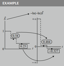
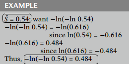
To illustrate the computation of a log-log value, suppose we start with an estimated survival probability of $0.54$. Then the log-log transformation of this value is $-\mathrm{ln} (-\mathrm{ln}0.54)$, which is $-\mathrm{ln}(0.616)$, because $\mathrm{ln}(0.54)$ equals $-0.616$. Now, $\mathrm{ln}(0.616)$ equals $-0.484$, because $\mathrm{ln}(0.616)$ equals $-0.484$. Thus, the transformation $-\mathrm{ln} (-\mathrm{ln}0.54)$ equals $0.484$.

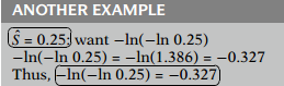
As another example, if the estimated survival probability is $0.25$, then $-\mathrm{ln} (-\mathrm{ln}0.25)$ equals $-\mathrm{ln}(1.386)$, which equals $-0.327$.

Why the PH assumption can be assessed by evaluating whether or not log-log curves are parallel.

Recall the formula for the survival curve that corresponds to the hazard function for the Cox PH model. Recall that there is a mathematical relationship between any hazard function and its corresponding survival function. We therefore can obtain the formula shown here for the survival curve for the Cox PH model. In this formula, the expression $S_0(t)$ denotes the baseline survival function that corresponds to the baseline hazard function $h_0(t)$.

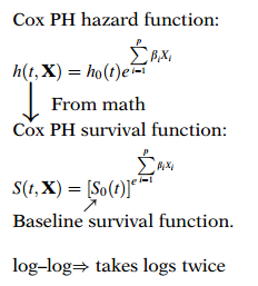
The log-log formula requires us to take logs of this survival function twice. The first time we take logs we get the expression shown here.

Now since $S(t, \mathbf{X})$ denotes a survival probability, its value for any $t$ and any specification of the vector $\mathbf{X}$ will be some number between 0 and 1. It follows that the natural log of any number between 0 and 1 is a negative number, so that the log of $S(t, \mathbf{X})$ as well as the log of $S_0(t)$ are both negative numbers. This is why we have to put a minus sign in front of this expression before we can take logs a second time, because there is no such thing as the log of a negative number.

Thus, when taking the second log, we must obtain the log of $-\mathrm{ln} S(t, \mathbf{X})$, as shown here. After using some algebra, this expression can be rewritten as the sum of two terms, one of which is the linear sum of the $\beta_iX_i$ and the other is the log of the negative log of the baseline survival function.

$\log \# 1:$

$$\begin{aligned} & \ln S(t, \mathbf{X})=e^{\sum_{i=1}^p \beta_i X_i} \times \ln S_0(t) \\ & 0 \leq S(t, \mathbf{X}) \leq 1 \end{aligned}$$

$\ln$ (probability) $=$ negative value, so $\ln S(t, \mathbf{X})$ and $\ln S_0(t)$ are negative. But $-\ln S(t, \mathbf{X})$ is positive, which allows us to take logs again.

$\log \# 2:$

$$\begin{aligned} \ln [ & -\ln S(t, \mathbf{X})] \\ = & \ln \left[-e^{\sum_{i=1}^p \beta_i X_i} \times \ln S_0(t)\right] \\ = & \ln \left[e^{\sum_{i=1}^p \beta_i X_i}\right]+\ln \left[-\ln S_0(t)\right] \\ = & \sum_{i=1}^p \beta_i X_i+\ln \left[-\ln S_0(t)\right] \\ & =\sum_{i=1}^p \beta_i X_i+\ln \left[-\ln S_0(t)\right] \end{aligned}$$

or

$$\begin{aligned} & -\ln [-\ln S(t, \mathbf{X})] \\ & =-\sum_{i=1}^p \beta_i X_i-\ln \left[-\ln S_0(t)\right] \end{aligned}$$

Now suppose we consider two different specifications of the $\mathbf{X}$ vector, corresponding to two different individuals, $\mathbf{X}_1$ and $\mathbf{X}_2$.

Two individuals:

$$\begin{aligned} & \mathbf{X}_1=\left(X_{11}, X_{12}, \ldots, X_{1 p}\right) \\ & \mathbf{X}_2=\left(X_{21}, X_{22}, \ldots, X_{2 p}\right) \\ \end{aligned}$$

Then the corresponding log-log curves for these individuals are given as shown here, where we have simply substituted $\mathbf{X}_1$ and $\mathbf{X}_2$ for $\mathbf{X}$ in the previous expression for the log-log curve for any individual $\mathbf{X}$.

$$\begin{aligned} & \left\{\begin{array}{l} \ln \left[-\ln S\left(t, \mathbf{X}_1\right)\right] \\ =\sum_{i=1}^p \beta_i X_{1 i}+\ln \left[-\ln S_0(t)\right] \\ \ln \left[-\ln S\left(t, \mathbf{X}_2\right)\right] \\ =\sum_{i=1}^p \beta_i X_{2 i}+\ln \left[-\ln S_0(t)\right] \\ \ln \left[-\ln S\left(t, \mathbf{X}_1\right)\right] \\ -\left(\ln \left[-\ln S\left(t, \mathbf{X}_2\right)\right]\right) \\ =\sum_{i=1}^p \beta_i\left(X_{1 i}-X_{2 i}\right) \end{array}\right. \end{aligned}$$

does not involve $t$

Subtracting the second log-log curve from the first yields the expression shown here. This expression is a linear sum of the differences in corresponding predictor values for the two individuals. Note that the baseline survival function has dropped out, so that the difference in log-log curves involves an expression that does not involve time $t$.

Alternatively, using algebra, we can write the above equation by expressing the log-log survival curve for individual $\mathbf{X}_1$ as the log-log curve for individual $\mathbf{X}_2$ plus a linear sum term that is independent of $t$.

$$\begin{aligned} & -\ln \left[-\ln S\left(t, \mathbf{X}_1\right)\right] \\ & =\ln \left[-\ln S\left(t, \mathbf{X}_2\right)\right] \\ & +\sum_{i=1}^p \beta_i\left(X_{1 i}-X_{2 i}\right) \end{aligned}$$

Therefore, if we use a Cox PH model and we plot the estimated log-log survival curves for individuals on the same graph, the two plots would be approximately parallel. The distance between the two curves is the linear expression involving the differences in predictor values, which does not involve time. Note, in general, if the vertical distance between two curves is constant, then the curves are parallel.

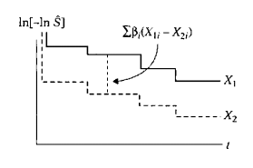
The parallelism of log-log survival plots for the Cox PH model provides us with a graphical approach for assessing the PH assumption. That is, if a PH model is appropriate for a given set of predictors, one should expect that empirical plots of log-log survival curves for different individuals will be approximately parallel.

Note: By empirical plots, we mean plotting log-log survival curves based on Kaplan-Meier (KM) estimates that do not assume an underlying Cox model.

Example

Consider the comparison of treatment and placebo groups in a clinical trial of leukemia patients, where survival time is time, in weeks, until a patient goes out of remission. Two predictors of interest in this study are treatment group status (1 = placebo, 0 = treatment), denoted as $R_x$, and log white blood cell count (log WBC), where the latter variable is being considered as a confounder.

To assess whether the PH assumption is satisfied for either or both of these variables, we would need to compare log-log survival curves involving categories of these variables.

One strategy to take here is to consider the variables one at a time. For the $R_x$ variable, this amounts to plotting log-log KM curves for treatment and placebo groups and assessing parallelism. If the two curves are approximately parallel, as shown here, we would conclude that the PH assumption is satisfied for the variable $R_x$. If the two curves intersect or are not parallel in some other way, we would conclude that the PH assumption is not satisfied for this variable.

For the log WBC variable, we need to categorize this variable into categories - say, low, medium, and high - and then compare plots of log-log KM curves for each of the three categories. In this illustration, the three log-log Kaplan-Meier curves are clearly nonparallel, indicating that the PH assumption is not met for log WBC.

---

Graphical Approach 2: Observed Versus Expected Plots

The use of observed versus expected plots to assess the PH assumption is the graphical analog of the goodness-of-fit (GOF) testing approach to be described later, and is therefore a reasonable alternative to the log-log survival curve approach.

As with the log-log approach, the observed versus expected approach may be carried out using either or both of two strategies-(1) assessing the PH assumption for variables one-at-a-time, or (2) assessing the PH assumption after adjusting for other variables. The strategy which adjusts for other variables uses a stratified Cox PH model to form observed plots, where the PH model contains the variables to be adjusted and the stratified variable is the predictor being assessed.

Here, we describe only the one-at-a-time strategy, which involves using KM curves to obtain observed plots.

Example

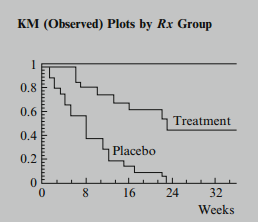
As an example, for the remission data on 42 leukemia patients we have illustrated earlier, the KM plots for the treatment and placebo groups, with 21 subjects in each group, are shown here. These are the "observed" plots.

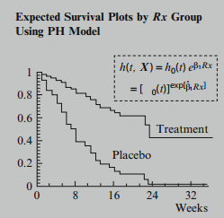
To obtain "expected" plots, we fit a Cox PH model containing the predictor being assessed. We obtain expected plots by separately substituting the value for each category of the predictor into the formula for the estimated survival curve, thereby obtaining a separate estimated survival curve for each category.

To compare observed with expected plots we then put both sets of plots on the same graph as shown here.

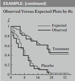
If observed and expected plots are:

• close, complies with PH assumption
• discrepant, PH assumption violated

---

The Goodness of Fit (GOF)Testing Approach

The implementation of the test can be thought of as a three-step process.

1. Run a Cox PH model and obtain Schoenfeld residuals for each predictor.

2. Create a variable that ranks the order of failures. The subject who has the first (earliest) event gets a value of 1, the next gets a value of 2, and so on.

3. Test the correlation between the variables created in the first and second steps. The null hypothesis is that the correlation between the Schoenfeld residuals and ranked failure time is zero.

   If p-value small, then departure from PH.

---

Assessing the PH Assumption Using Time-Dependent Covariates

A. Use extended Cox model: contains product terms of form $X \times g(t)$, where $g(t)$ is function of time, e.g., $g(t)=t$, or $\log t$, or heaviside function.

B. One-at-a-time model:

$$h(t, \mathbf{X})=h_0(t) \exp [\beta X+\delta X g(t)]$$

Test $H_0: \delta=0$ using Wald or LR test (chi- square with $1 \mathrm{df})$.

C. Evaluating several predictors simultaneously:

$$h(t, \mathbf{X})=h_0(t) \exp \left(\sum_{i=1}^p\left[\beta_i X_i+\delta_i X_i g_i(t)\right]\right)$$

where $g_i(t)$ is function of time for $i$ th predictor.

Test $H_0: \delta_1=\delta_2=\cdots=\delta_p=0$ using $L R$ (chi-square) test with $p$ df.

Drawback:

1. choice of $g(t)$ not always clear
2. different choices may lead to different conclusions about $\mathrm{PH}$ assumption.